
Capped means, exposure curves and increased limit factors
Source:vignettes/CappedMean.Rmd
CappedMean.Rmd1.Introduction
This vignette will cover capped mean functions, exposure and increased limit factor curves of the NetSimR package. It will overview the theory behind these functions, propose possible uses and illustrate examples. The distributions covered for claim severities are LogNormal, Gamma, Pareto, Sliced LogNormal-Pareto, Sliced Gamma-Pareto. An application of the capped mean is suggested in the article “Taken to excess” accessible here.
2.Background theory
Let claim severity originate from a probability density function and a cumulative density function . Let claims be capped at amount . The capped claim severity is defined as .
2.1 Capped mean
The expected mean can be estimated by: The expected capped claim can be obtained by: The above simplifies to: This equation will need to be solved for every distribution.
3. Functions usage
In this section we will suggest possible uses of the specified functions.
3.1 Capped mean
- Restricting expected claims from being modelled beyond the property’s value, in property lines.
- Modelling attritional losses with a censored or truncated distribution, in order to improve our estimate. Large claims will be modelled separately. This can be extended to Generalised Linear Models.
- Estimating the cost of deductibles.
- Pricing reinsurance excess of loss layers.
3.2 Exposure curve
For property lines/sections:
- Pricing/allocating premium of excess of loss layers.
- Loading for large losses.
Note: for property lines, instead of severity, we may opt to model severity as a percentage of sum insured. In GLMs this is equivalent to having the sum insured as the exposure for the severity distribution.
4. Examples
4.1 Capped mean
The below code illustrates an alternative and more accurate approach to applying capping in regressions, for modelling attritional claims part. The code steps are:
- Simulate 10,000 claims
- Cap the claims
- Fit a lognormal regression to the capped claims
- Fit a censored regression to the capped claims
- Compare:
- the expected mean from the normal regression
- the expected capped mean from the censored regression
- the mean of the capped claims data
The example suggests that the proposed method outperforms the market approach on LogNormal distribution. The one-way benefit will not be significant on a Gamma distribution, but when we move to a GLM and the model relativities are larger, the capped mean benefit may also be significant.
library("NetSimR")

#Set parameters
n<-10000
mu<-6
sigma<-1.7
Cap <- 10000

#Set seed to keep simulations constant
set.seed(10)

#Simulate data
x<-round(rlnorm(n,mu,sigma),0)
head(x)
## [1] 416 295 39 146 666 783
summary(x)## Min. 1st Qu. Median Mean 3rd Qu. Max.
## 1 128 400 1769 1279 263389
plot(x)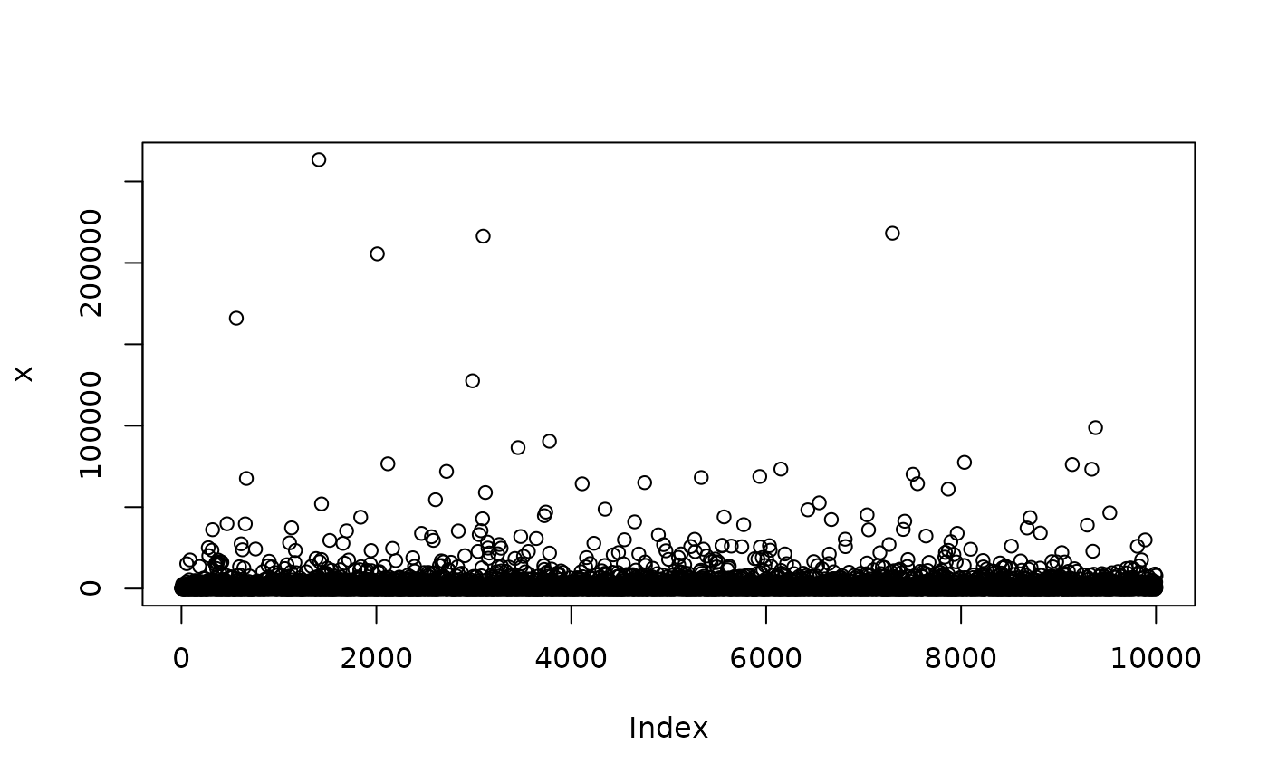
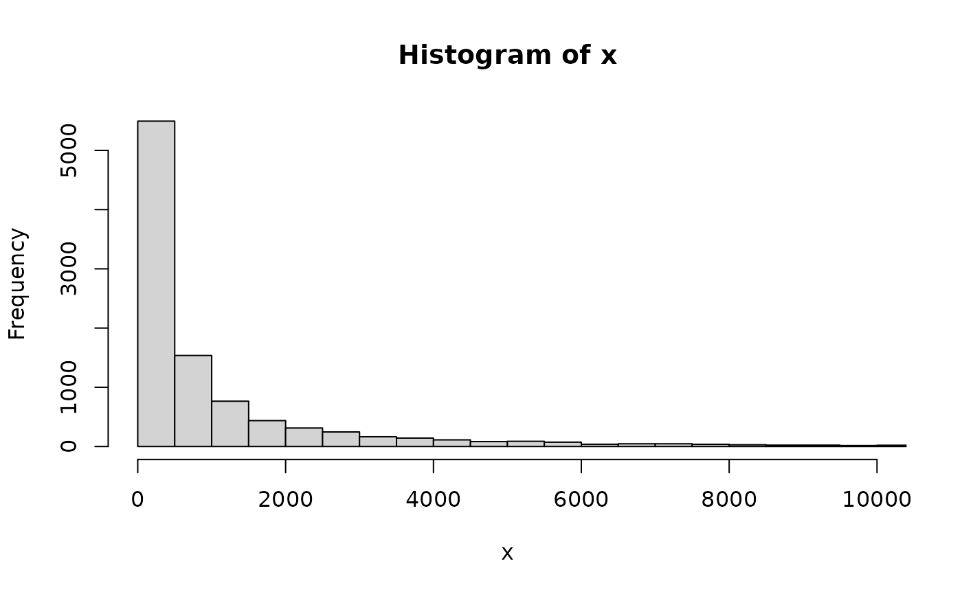
## [1] 416 295 39 146 666 783
summary(z)## Min. 1st Qu. Median Mean 3rd Qu. Max.
## 1 128 400 1282 1279 10000
plot(z)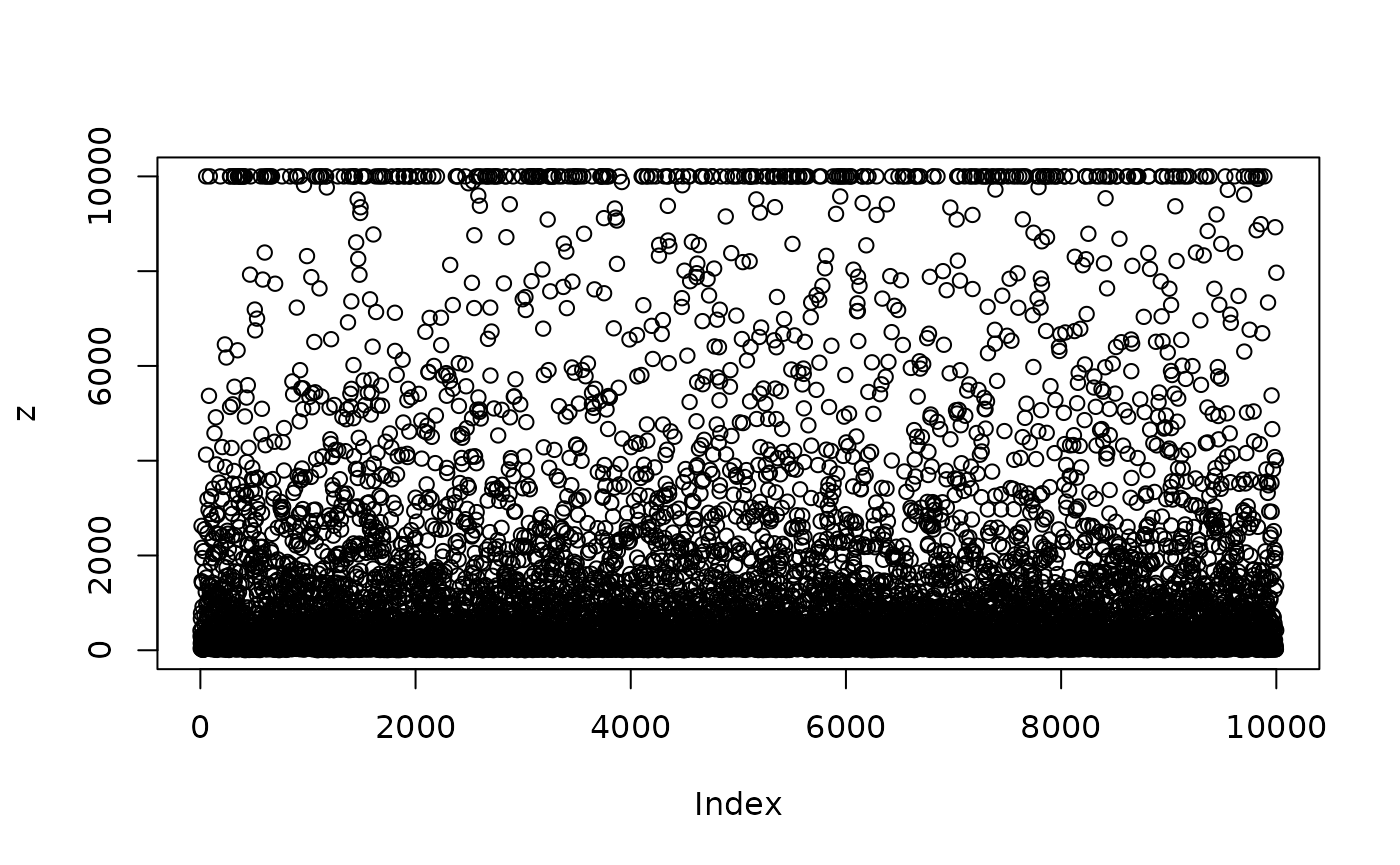
hist(z, breaks = 200)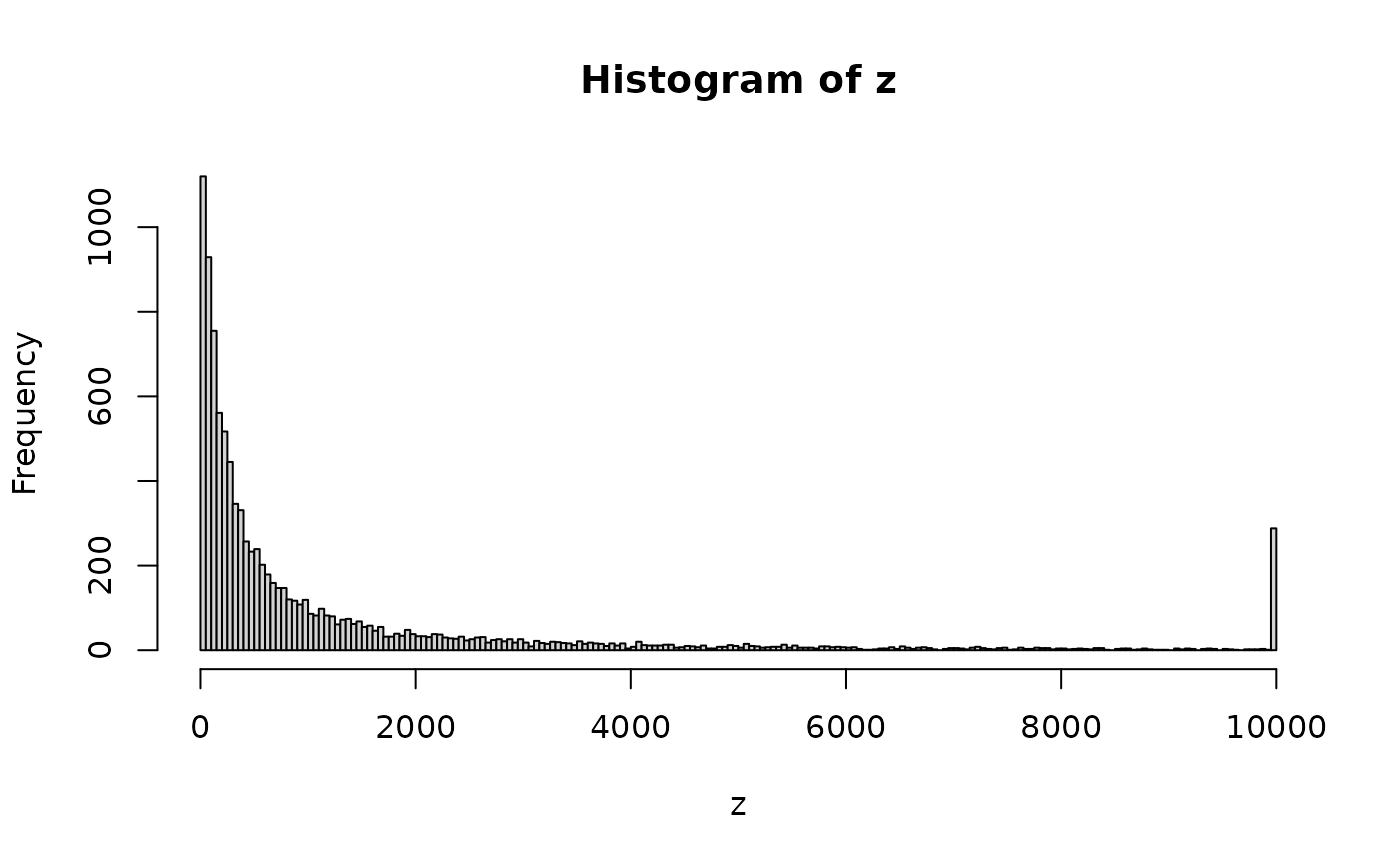
##
## Call:
## lm(formula = log(z) ~ 1)
##
## Residuals:
##     Min      1Q  Median      3Q     Max
## -5.9815 -1.1295  0.0099  1.1723  3.2288
##
## Coefficients:
##             Estimate Std. Error t value Pr(>|t|)
## (Intercept)  5.98153    0.01662   359.8   <2e-16 ***
## ---
## Signif. codes:  0 '***' 0.001 '**' 0.01 '*' 0.05 '.' 0.1 ' ' 1
##
## Residual standard error: 1.662 on 9999 degrees of freedom
#fit a right censored normal model to log(z) by maximum likelihood: an uncapped claim
#contributes its density, a capped one the probability of a claim above the cap
censoredLogLik <- function(par, y, cap) {
  mu <- par[1]
  sigma <- exp(par[2])
  capped <- y >= cap
  sum(dnorm(y[!capped], mu, sigma, log = TRUE)) +
    sum(capped) * pnorm(cap, mu, sigma, lower.tail = FALSE, log.p = TRUE)
}
fit <- optim(c(mean(log(z)), log(sd(log(z)))), function(par) -censoredLogLik(par, log(z), log(Cap)),
             method = "BFGS")
censored <- c(mu = fit$par[1], sigma = exp(fit$par[2]))


#Compare regression outputs
cbind(coefficients(lmLinear),summary(lmLinear)$sigma)
## [,1] [,2]
## (Intercept) 5.981527 1.662243
censored## mu sigma
## 6.000536 1.705256
#Compare regressions' attritional capped cost to empirical
round(cbind(
  Empirical=mean(z)
  ,LinearModel=exp(coefficients(lmLinear)+0.5*summary(lmLinear)$sigma*summary(lmLinear)$sigma)
  ,CensoredModel=LNormCappedMean(Cap,censored[["mu"]],censored[["sigma"]])
),0)
## Empirical LinearModel CensoredModel
## (Intercept) 1282 1577 1284Modelling excess levels would be similar to the above approach. In that case the expected mean above the excess levels would be the mean less the expected mean below the excess level. This is elaborated in the article cited in the introduction section.
4.2 Exposure curve
For a LogNormal severity, generating the exposure curve value at a particular point is obtained by running the below code:
ExposureCurveLNorm(1000,5,1.6)## [1] 0.5601327This would be interpreted as: 56% of the expected cost is up to 1,000 currency units. Other distributions follow the same logic. The challenge for this exercise would be fitting the correct severity distribution, rather than calculating the Exposure curve’s value.
4.3 Increased limit factor curve
For a LogNormal severity, generating the increased limit factor value between two particular points is obtained by running the below code:
ILFLNorm(1000,1500,5,1.6)## [1] 1.155086This would be interpreted as: the expected cost of the claims up to 1,500 currency units is 1.155 times the expected cost of the claims up to 1,000 currency units. Other distributions follow the same logic. The challenge for this exercise would be fitting the severity distribution, rather than calculating the Increased Limit Factor curve’s value.