
1. Introduction
This vignette prices a layer of an excess of loss treaty: 4 million excess of 1 million, each and every loss, with one reinstatement at 100%, for the year 2025. It rates the layer on its loss experience, with the burning cost and a Pareto model of the large losses, then on its exposure, with a risk profile and an exposure curve, blends the two and turns the expected loss into a premium.
Every step here also runs in the reinsurance pricing tool,
run_shiny_reinsurance_pricing_tool(), which can be tried in
the browser on the package’s website.
2. The experience
xl_large_losses holds the large losses of a simulated
portfolio from 2015 to 2024, those of at least 500,000 in the money of
their year, and xl_premium the subject premium of each
year, with a rate index that brings it to the rates of 2025 and the
development factor of its layer losses:
##      claim year  amount
## 1 C2015-01 2015 5477300
## 2 C2015-02 2015  798900
## 3 C2015-03 2015  696600
## 4 C2015-04 2015  552700
## 5 C2015-05 2015  534100
## 6 C2016-01 2016  910700
xl_premium## year premium rate_index development
## 1 2015 41200000 0.94 1.00
## 2 2016 42500000 0.96 1.00
## 3 2017 43100000 0.99 1.00
## 4 2018 44800000 1.02 1.01
## 5 2019 46000000 1.05 1.02
## 6 2020 47900000 1.06 1.04
## 7 2021 50600000 1.04 1.08
## 8 2022 53200000 1.03 1.15
## 9 2023 55800000 1.01 1.30
## 10 2024 58400000 1.00 1.653. The burning cost
burning_cost() brings each loss to the money of 2025
with the claims inflation, takes its part in the layer, develops each
year’s layer losses to ultimate, applies the annual aggregate limit (two
limits, with one reinstatement) and divides by the year’s on-level
premium:
development <- setNames(xl_premium$development, xl_premium$year)
rate_index <- setNames(xl_premium$rate_index, xl_premium$year)
premium <- xl_premium[, c("year", "premium")]
bc <- burning_cost(xl_large_losses, premium, deductible = 1e6, limit = 4e6, aggregate_limit = 8e6,
                   inflation = 0.04, rating_year = 2025, development = development,
                   premium_index = rate_index, threshold = 5e5, rating_premium = 60e6)
bc
## Burning cost of 4,000,000 xs 1,000,000 for 2025
## Years: 10 (2015 to 2024)
## Losses in the layer: 25
## Burning cost: 4.972% of subject premium (premium weighted)
## Expected layer loss: 2,983,162
bc$by_year[, c("year", "layer_count", "aggregate_losses", "onlevel_premium", "burning_cost")]## year layer_count aggregate_losses onlevel_premium burning_cost
## 1 2015 3 4213705.3 38728000 0.108802554
## 2 2016 2 550147.8 40800000 0.013484014
## 3 2017 0 0.0 42669000 0.000000000
## 4 2018 2 445862.7 45696000 0.009757150
## 5 2019 5 6403567.0 48300000 0.132579026
## 6 2020 1 46782.5 50774000 0.000921387
## 7 2021 4 4393616.6 52624000 0.083490738
## 8 2022 4 5627256.8 54796000 0.102694664
## 9 2023 3 2034220.0 56358000 0.036094610
## 10 2024 1 604824.0 58400000 0.010356575The threshold of the data matters: a loss just below 500,000 in 2015
is about 740,000 in the money of 2025. Had the deductible been below the
indexed threshold, losses missing from the data could have reached the
layer, and burning_cost() would have warned.
4. The Pareto model
The burning cost rests on the few losses that reached the layer, and
it cannot price a layer above the largest loss seen.
pareto_rating() fits a Pareto distribution to the indexed
losses above a threshold and prices the layer from the frequency of
large losses and their expected part in the layer. The threshold must be
at least the reporting threshold indexed from the oldest year, here
about 740,000: below it, the oldest years lack the losses that were
under 500,000 in their own money, and the fitted alpha comes out too
low. So the threshold is 750,000:
pr <- pareto_rating(xl_large_losses, premium, threshold = 7.5e5, deductible = 1e6, limit = 4e6,
                    inflation = 0.04, rating_year = 2025, development = development,
                    premium_index = rate_index, rating_premium = 60e6)
pr
## Pareto rating of 4,000,000 xs 1,000,000 for 2025
## Threshold: 750,000
## Losses above it: 34
## Alpha: 1.567
## Rate: 5.115% of subject premium
## Expected count: 4.56 losses above the threshold
## Expected layer loss: 3,068,752A market alpha can replace the one estimated with
alpha =, which is how a thin experience is often
priced.
5. Exposure rating
Exposure rating needs no loss experience.
xl_property_profile is the risk profile of a property
portfolio: bands of sum insured with their premium. With an expected
loss ratio of 55%, each band’s expected loss is shared between the layer
and the rest by an exposure curve, here Swiss Re’s Y3 curve
(mbbefd_curve(), swiss_re_curve()):
exposure <- property_exposure_rating(xl_property_profile, deductible = 1e6, limit = 4e6,
                                     curve = "Y3", loss_ratio = 0.55)
exposure
## Exposure rating (property) of 4,000,000 xs 1,000,000
## Curve: Swiss Re Y3 (c = 3)
## Bands: 9
## Subject premium: 57,227,000
## Ground-up loss: 31,474,850
## Expected layer loss: 3,705,907
## Rate: 6.476% of subject premium
exposure$bands[, c("band", "sum_insured", "deductible_share", "exhaustion_share", "layer_share", "layer_loss")]## band sum_insured deductible_share exhaustion_share layer_share
## 1 0 to 250k 138000 1.00000000 1.00000000 0.0000000
## 2 250k to 500k 382000 1.00000000 1.00000000 0.0000000
## 3 500k to 1m 750000 1.00000000 1.00000000 0.0000000
## 4 1m to 2.5m 1715000 0.58309038 1.00000000 0.1788200
## 5 2.5m to 5m 3638000 0.27487631 1.00000000 0.3774279
## 6 5m to 10m 7200000 0.13888889 0.69444444 0.4035249
## 7 10m to 25m 16450000 0.06079027 0.30395137 0.3317604
## 8 25m to 50m 34875000 0.02867384 0.14336918 0.2767503
## 9 50m to 100m 69000000 0.01449275 0.07246377 0.2221608
## layer_loss
## 1 0.00
## 2 0.00
## 3 0.00
## 4 897354.50
## 5 1129056.65
## 6 805415.62
## 7 528245.44
## 8 254804.03
## 9 91030.37The curves run from Y1, for personal lines, where most losses are small against the sum insured, to Y4 for large industrial risks; the Lloyd’s curve (c = 5) has more total losses still:
x <- seq(0, 1, by = 0.01)
plot(x, swiss_re_curve(x, "Y1"), type = "l", xlab = "Deductible as a share of the sum insured",
     ylab = "Share of the expected loss below it")
for (c in c("Y2", "Y3", "Y4", "Lloyds")) lines(x, swiss_re_curve(x, c))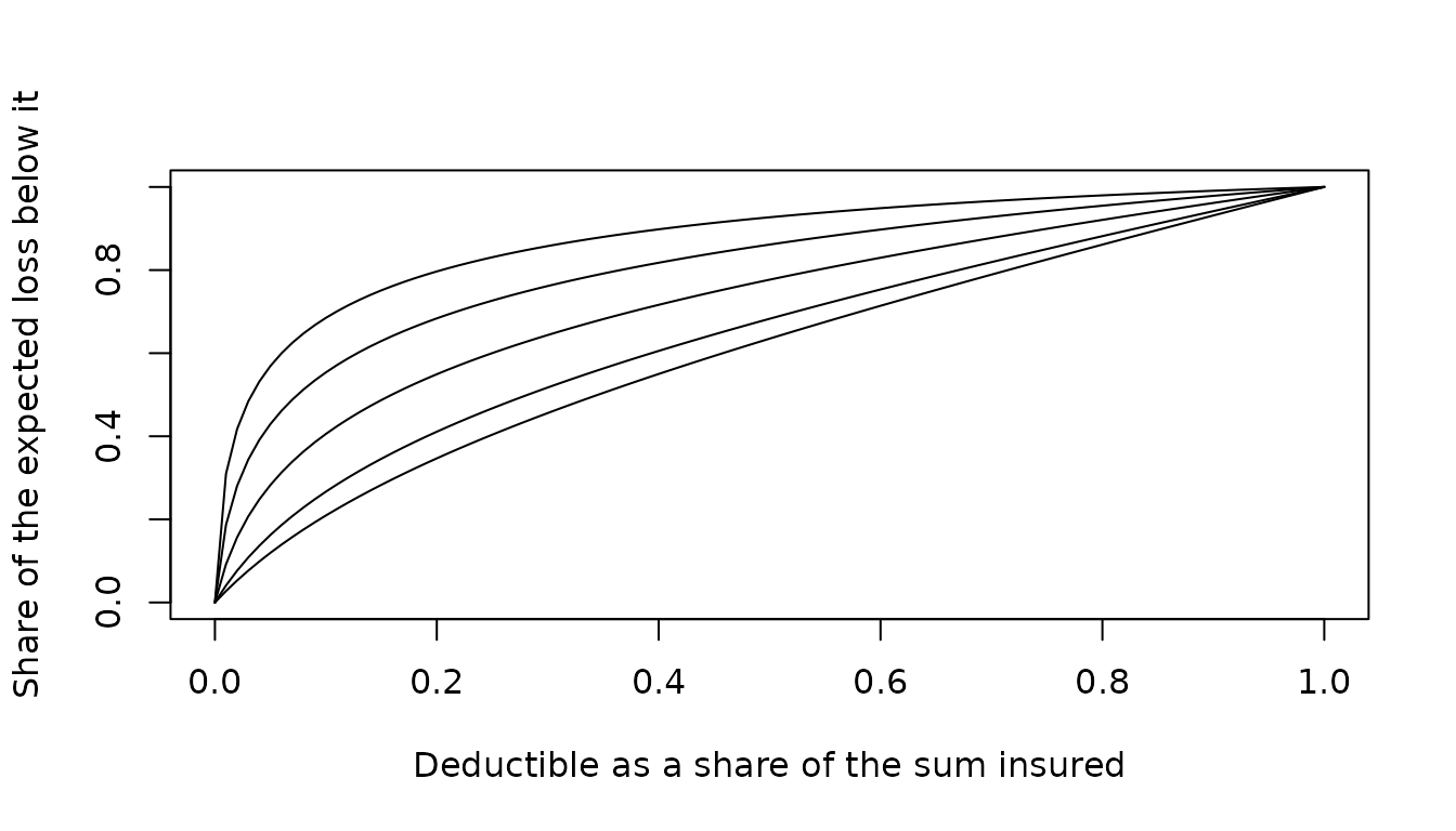
For casualty business, casualty_exposure_rating() does
the same with the policy limits of the profile and a claim size
distribution, such as one fitted with the distribution fitting tool:
casualty_exposure_rating(xl_casualty_profile, deductible = 1e6, limit = 4e6, severity = "LogNormal",
                         severity_params = c(meanlog = 10, sdlog = 2), loss_ratio = 0.65)
## Exposure rating (casualty) of 4,000,000 xs 1,000,000
## Curve: Log-Normal (meanlog = 10, sdlog = 2)
## Bands: 6
## Subject premium: 49,000,000
## Ground-up loss: 31,850,000
## Expected layer loss: 3,298,205
## Rate: 6.731% of subject premium6. Blending and the premium
The experience and exposure rates are blended with a credibility weight. Limited fluctuation credibility gives the experience the weight for losses in the layer; the standard of 1,082 losses for full credibility is a strict one for a layer, and a lower one is often chosen:
z <- credibility_weight(bc$n_layer_losses, full = 100)
z
## [1] 0.5
rate <- z * bc$rate + (1 - z) * exposure$rate
expected_loss <- rate * 60e6
expected_loss
## [1] 3434321technical_premium() loads the expected loss for
expenses, brokerage and profit: the upfront premium and the expected
reinstatement premium together are the expected loss over one minus the
loading. The reinstatement premium depends on how much of the reinstated
cover is used each year. This is a working layer, whose losses some
years exceed the one reinstated limit, so the expected loss over the
limit would overstate it; the burning cost’s years, at the rating year’s
premium and scaled to the blended expected loss, give a better
estimate:
years <- bc$by_year$at_rating_premium * expected_loss / bc$expected_loss
used <- mean(pmin(years, 1 * 4e6)) / 4e6
used
## [1] 0.5219395
premium <- technical_premium(expected_loss, limit = 4e6, loading = 0.25, reinstatements = 1,
                             reinstatement_rate = 1, used = used)
premium
## $expected_loss
## [1] 3434321
##
## $total_premium
## [1] 4579095
##
## $upfront_premium
## [1] 3008724
##
## $reinstatement_premium
## [1] 1570372
##
## $rate_on_line
## [1] 0.7521809
##
## $payback
## [1] 1.329467
##
## $used
## [1] 0.5219395The upfront premium is 75% of the limit, a rate on line typical of a
working layer, which pays back the limit in 1.3 years. For the
distribution of the layer’s annual losses and reinstatement premiums,
simulate the portfolio with simulate_claims(), using the
Pareto fitted here for the large losses.