
1.Introduction
This vignette shows how to simulate insurance claims with
simulate_claims(). For each simulated period (for example a
year) the function draws the number of claims from a frequency
distribution and the size of each claim from a severity distribution. It
can replace the tail of the severity with Pareto slices, cap each claim,
and apply an each-and-every-loss layer (with limited reinstatements) and
an aggregate layer. It returns one row per period.
The same model runs in the claims simulator app,
run_shiny_simulator(), and through
simulate_function(), which has the app’s long argument
names. simulate_claims() has short names and defaults for
everything optional.
The runs below are kept small so that the vignette builds quickly. At least 10,000 simulations are recommended for figures at the 99.5% level.
2. A first run
5,000 periods with a Poisson number of claims (3 a year on average) and Log-Normal claim sizes:
library("NetSimR")

claims <- simulate_claims(
  5000, frequency = "Poisson", frequency_params = 3,
  severity = "LogNormal", severity_params = c(8, 1.5), seed = 1
)
head(claims)
## claim_counts total_claims gross_claims
## 1 4 159368.374 159368.374
## 2 3 2895.332 2895.332
## 3 5 8970.495 8970.495
## 4 6 14026.745 14026.745
## 5 5 26582.006 26582.006
## 6 2 6760.205 6760.205claim_counts is the number of claims in each period,
total_claims the total after any layers and
gross_claims the total before them. Without layers the two
are the same.
A small helper gives the usual summary statistics: the mean, the standard deviation, the 99.5% Value at Risk (VaR, the loss exceeded once in 200 periods) and the 99.5% Tail Value at Risk (TVaR, the average of the worst 0.5% of periods).
tail_stats <- function(x) {
  worst <- sort(x, decreasing = TRUE)[seq_len(ceiling(0.005 * length(x)))]
  c(mean = mean(x), sd = sd(x), VaR99.5 = unname(quantile(x, 0.995)), TVaR99.5 = mean(worst))
}
round(tail_stats(claims$total_claims))
## mean sd VaR99.5 TVaR99.5
## 28009 52982 284160 502727
# the expected total is the mean number of claims times the mean claim size
3 * exp(8 + 1.5^2 / 2)
## [1] 27545.99
hist(claims$total_claims, breaks = 100, main = "Total claims per period", xlab = "Total claims")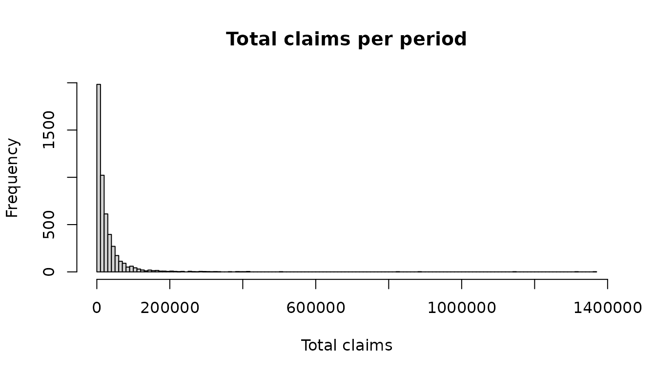
3. Distributions and their parameters
The frequency can be Poisson, Negative Binomial, Binomial, a
zero-inflated Poisson or Negative Binomial (section 4), or a fixed
number of claims; the severity Normal, Log-Normal, Gamma, Exponential,
Pareto, Weibull, Burr, generalised Pareto (section 5) or a fixed amount.
The table in ?simulate_claims lists the parameters of each.
Names ignore case, spaces and underscores, and the parameters can be
given in order or named, in any order:
named <- simulate_claims(
  5000, frequency = "negative binomial", frequency_params = c(beta = 1.5, r = 2),
  severity = "gamma", severity_params = c(shape = 2, scale = 5000), seed = 1
)
in_order <- simulate_claims(5000, "Negative_Binomial", c(2, 1.5), "Gamma", c(2, 5000), seed = 1)
identical(named, in_order)
## [1] TRUE4. Zero-inflated claim counts
Some portfolios have more periods without any claim than a Poisson or
a Negative Binomial allows: a cover that is only sometimes exposed, a
large-loss or catastrophe layer, a scheme that is dormant in some years.
A zero-inflated count is zero with probability zero_prob,
and otherwise drawn from the Poisson (or the Negative Binomial) of its
other parameters. With a Poisson of mean
and a probability
of an extra zero, the mean is
,
the variance
,
and the chance of no claim
.
Here 40% of the periods are extra zeros and the others have 5 claims on average, so the mean is 3 claims a period, as in the first run:
zero_inflated <- simulate_claims(
  5000, frequency = "Zero-inflated Poisson", frequency_params = c(lambda = 5, zero_prob = 0.4),
  severity = "LogNormal", severity_params = c(8, 1.5), seed = 1
)
count_stats <- function(n) c(mean = mean(n), variance = var(n), no_claims = mean(n == 0))
round(rbind(
  poisson = count_stats(claims$claim_counts),
  zero_inflated = count_stats(zero_inflated$claim_counts),
  zero_inflated_expected = c(0.6 * 5, 0.6 * 5 * (1 + 0.4 * 5), 0.4 + 0.6 * exp(-5))
), 3)
## mean variance no_claims
## poisson 3.008 3.078 0.053
## zero_inflated 2.975 8.901 0.404
## zero_inflated_expected 3.000 9.000 0.404The counts have the same mean but three times the variance, and two periods in five have no claim. The total claims are only a little more volatile, as here the claim sizes, not the counts, drive most of their volatility:
round(rbind(poisson = tail_stats(claims$total_claims), zero_inflated = tail_stats(zero_inflated$total_claims)))## mean sd VaR99.5 TVaR99.5
## poisson 28009 52982 284160 502727
## zero_inflated 27781 56781 284340 505901"Zero-inflated Negative Binomial" takes r,
beta and zero_prob. The distribution fitting
tool, run_shiny_distribution_fitting_tool(), fits both to
claim counts beside the Poisson and the Negative Binomial, and suggests
the one with the lowest AIC: a zero-inflated model is worth its extra
parameter only when the data has more zeros than the others give.
5. Weibull, Burr and generalised Pareto claim sizes
Three more severities have tails of other kinds than the Log-Normal’s:
- the Weibull, with a
shapeand ascale: . A shape below 1 gives a tail heavier than that of the Exponential, but lighter than any Pareto tail; - the Burr (type XII), with
alpha,gammaand ascale: . It has a Pareto tail of index over a body shaped by ( is the Lomax, the log-logistic); - the generalised Pareto, with a
location, ascaleand ashape: above its location. It has a Pareto tail of index for a positive shape, and is the Exponential for a shape of 0. It is the distribution extreme value theory gives for the claims above a high threshold, its location.
The tail index is the alpha of the Pareto the tail follows: the lower it is, the heavier the tail, and moments of that order and above are infinite. To compare the four, each is given the mean claim of the Log-Normal of the first run, from the formula of its mean:
mean_claim <- exp(8 + 1.5^2 / 2)
severities <- list(
  LogNormal = list("LogNormal", c(8, 1.5)),
  # mean: scale * gamma(1 + 1 / shape)
  Weibull = list("Weibull", c(shape = 0.6, scale = mean_claim / gamma(1 + 1 / 0.6))),
  # mean: scale * alpha * beta(alpha - 1 / gamma, 1 + 1 / gamma); tail index 1.5 * 1.5 = 2.25
  Burr = list("Burr", c(alpha = 1.5, gamma = 1.5, scale = mean_claim / (1.5 * beta(1.5 - 1 / 1.5, 1 + 1 / 1.5)))),
  # mean: location + scale / (1 - shape); tail index 1 / 0.4 = 2.5
  `Generalised Pareto` = list("Generalised Pareto", c(location = 0, scale = mean_claim * (1 - 0.4), shape = 0.4))
)
runs <- lapply(severities, function(s) simulate_claims(20000, "Poisson", 3, s[[1]], s[[2]], seed = 1))
round(t(sapply(runs, function(r) tail_stats(r$total_claims))))
## mean sd VaR99.5 TVaR99.5
## LogNormal 27309 46055 271405 425194
## Weibull 27609 32573 177785 222003
## Burr 27680 38629 169907 307638
## Generalised Pareto 27706 41670 198612 344855The means agree, as they should; the differences are in the tail. The Weibull has the lowest TVaR: its tail is the lightest. The Burr’s 99.5% VaR is below the Weibull’s but its TVaR well above, as its Pareto tail shows beyond that level. And the Log-Normal with a sigma of 1.5 is the heaviest of the four at this level, although it has no Pareto tail: a tail index says which distribution is the heavier far enough out, not at a given return period. Which one fits is a question for the data: the distribution fitting tool fits all of them by maximum likelihood (also to claims reported above a threshold, or capped at policy limits), compares them by the Kolmogorov-Smirnov distance, the Anderson-Darling statistic and the AIC, and draws a Hill plot of the tail index. Its Export tab saves the fitted model as a settings file for the claims simulator and for the Programmes tab of the reinsurance pricing tool.
6. A Pareto tail
Rather than choosing one distribution for all claim sizes, the tail
of any severity can be replaced. Log-Normal tails are often too light
for large claims. pareto_thresholds and
pareto_alphas replace the tail above each threshold with a
Pareto distribution; here claims above 100,000 follow a Pareto with
alpha 1.5. Up to six slices can be given, with increasing
thresholds.
tail <- simulate_claims(
  5000, "Poisson", 3, "LogNormal", c(8, 1.5), seed = 1,
  pareto_thresholds = 100000, pareto_alphas = 1.5
)
round(rbind(lognormal = tail_stats(claims$total_claims), pareto_tail = tail_stats(tail$total_claims)))
## mean sd VaR99.5 TVaR99.5
## lognormal 28009 52982 284160 502727
## pareto_tail 31022 108770 410076 953869The severity is then the sliced Log-Normal-Pareto distribution of the “Sliced LogNormal-Pareto and Gamma-Pareto distributions” vignette, so its mean gives the expected total. With alpha 1.5 the variance is infinite, so the simulated mean converges slowly.
c(expected = 3 * SlicedLNormParetoMean(8, 1.5, 100000, 1.5), simulated = mean(tail$total_claims))## expected simulated
## 30671.80 31021.78A return-period chart shows where the two models differ:
return_periods <- function(x) data.frame(rp = 1 / (1 - ppoints(length(x))), loss = sort(x))
lognormal_rp <- return_periods(claims$total_claims)
pareto_rp <- return_periods(tail$total_claims)
keep <- lognormal_rp$rp <= 500
plot(loss ~ rp, data = pareto_rp[keep, ], type = "l", log = "x", col = "firebrick", lwd = 2,
     xlab = "Return period (years)", ylab = "", yaxt = "n")
axis(2, at = axTicks(2), labels = format(axTicks(2), big.mark = ",", scientific = FALSE), las = 1, cex.axis = 0.8)
lines(loss ~ rp, data = lognormal_rp[keep, ], col = "steelblue", lwd = 2)
legend("topleft", c("Pareto tail above 100,000", "Log-Normal"), col = c("firebrick", "steelblue"), lwd = 2, bty = "n")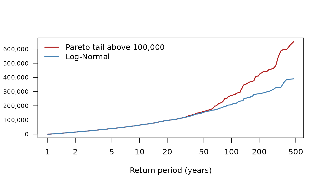
7. An each-and-every-loss layer with reinstatements
An each-and-every-loss (EEL) layer applies to every claim. A
“limited” layer of 50,000 excess of 20,000 pays
min(max(claim - 20000, 0), 50000) for each claim; with two
reinstatements it pays at most (2 + 1) * 50000 = 150000 in
a period.
layer <- simulate_claims(
  5000, "Poisson", 3, "LogNormal", c(8, 1.5), seed = 1,
  pareto_thresholds = 100000, pareto_alphas = 1.5,
  eel_layer = "limited", eel_deductible = 20000, eel_limit = 50000,
  eel_reinstatements = 2
)
head(layer)
## claim_counts total_claims gross_claims number_of_reinstatements_used
## 1 4 50000 221252.193 1
## 2 3 0 2895.332 0
## 3 5 0 8970.495 0
## 4 6 0 14026.745 0
## 5 5 0 26582.006 0
## 6 2 0 6760.205 0total_claims is now the loss ceded to the layer and
gross_claims the loss before it, so the net loss is their
difference. number_of_reinstatements_used is the layer’s
recoveries in the period divided by the limit, capped at the number of
reinstatements.
# amounts ceded to the layer
round(c(largest = max(layer$total_claims), expected_loss = mean(layer$total_claims)))
## largest expected_loss
## 147460 6262
# probabilities, and the expected loss as a share of the limit
round(c(
  chance_hit = mean(layer$total_claims > 0),
  loss_on_line = mean(layer$total_claims) / 50000,
  chance_all_reinstatements_used = mean(layer$number_of_reinstatements_used >= 2)
), 4)
## chance_hit loss_on_line
## 0.2652 0.1252
## chance_all_reinstatements_used
## 0.0012
# the net (retained) losses
round(tail_stats(layer$gross_claims - layer$total_claims))
## mean sd VaR99.5 TVaR99.5
## 24759 102977 352795 894456The other layer types are “unlimited” (everything above the deductible) and “exclude” (the claims with the layer taken out, i.e. the retained losses).
8. An aggregate deductible
An aggregate layer applies to each period’s total after the EEL layer. The order is: severity cap, EEL layer on each claim, sum over the period, aggregate deductible, then the aggregate limit and the reinstatement capacity. So the aggregate deductible comes off the layer’s recoveries before the reinstatement capacity caps them.
For example, three claims of 100 through a layer of 100 excess of 0 with no reinstatements, and an aggregate deductible of 50: the layer recovers 300, the deductible leaves 250, and the capacity of one limit caps that at 100.
simulate_claims(
  3, frequency = "Fixed_number_of_Counts", frequency_params = 3,
  severity = "Fixed_Severity", severity_params = 100,
  eel_layer = "limited", eel_deductible = 0, eel_limit = 100, eel_reinstatements = 0,
  agg_layer = "unlimited", agg_deductible = 50
)
## claim_counts total_claims gross_claims number_of_reinstatements_used
## 1 3 100 300 0
## 2 3 100 300 0
## 3 3 100 300 0An annual aggregate deductible of 25,000 on the layer of section 7 reduces its expected loss. With the same seed the claims are the same, so the difference comes from the deductible alone:
with_deductible <- simulate_claims(
  5000, "Poisson", 3, "LogNormal", c(8, 1.5), seed = 1,
  pareto_thresholds = 100000, pareto_alphas = 1.5,
  eel_layer = "limited", eel_deductible = 20000, eel_limit = 50000,
  eel_reinstatements = 2, agg_layer = "unlimited", agg_deductible = 25000
)
c(without = mean(layer$total_claims), with = mean(with_deductible$total_claims))
## without with
## 6262.340 2203.6489. Faster runs with gross = FALSE
When only the ceded losses of an “unlimited” or “limited” EEL layer
are needed, gross = FALSE draws only the claims that reach
the layer, which is much faster for a high deductible. Here only about
one claim in 10 is above 20,000:
1 - pSlicedLNormPareto(20000, 8, 1.5, 100000, 1.5)## [1] 0.102222The results follow the same distribution, but they are not the same
draws as with gross = TRUE, and there is no
gross_claims column:
fast <- simulate_claims(
  20000, "Poisson", 3, "LogNormal", c(8, 1.5), seed = 1,
  pareto_thresholds = 100000, pareto_alphas = 1.5,
  eel_layer = "limited", eel_deductible = 20000, eel_limit = 50000,
  eel_reinstatements = 2, gross = FALSE
)
names(fast)
## [1] "claim_counts" "total_claims"
## [3] "number_of_reinstatements_used"
full <- simulate_claims(
  20000, "Poisson", 3, "LogNormal", c(8, 1.5), seed = 1,
  pareto_thresholds = 100000, pareto_alphas = 1.5,
  eel_layer = "limited", eel_deductible = 20000, eel_limit = 50000,
  eel_reinstatements = 2
)
round(rbind(gross_false = tail_stats(fast$total_claims), gross_true = tail_stats(full$total_claims)))
## mean sd VaR99.5 TVaR99.5
## gross_false 6286 14917 69711 88241
## gross_true 6296 14898 73302 9006710. Reproducible runs
A seed makes a run reproducible, and leaves the random
number stream of the session unchanged. Without a seed,
set.seed() before the call has the same effect:
a <- simulate_claims(2000, "Poisson", 3, "Gamma", c(2, 5000), seed = 42)
b <- simulate_claims(2000, "Poisson", 3, "Gamma", c(2, 5000), seed = 42)
identical(a, b)
## [1] TRUE
set.seed(42)
c1 <- simulate_claims(2000, "Poisson", 3, "Gamma", c(2, 5000))
set.seed(42)
c2 <- simulate_claims(2000, "Poisson", 3, "Gamma", c(2, 5000))
identical(c1, c2)
## [1] TRUEThe simulations run in chunks, and each chunk draws from its own
random stream derived from the seed. So parallel = TRUE,
which runs the chunks on worker R processes, gives exactly the same
results as a sequential run. By default each call starts one worker per
core and shuts them down when it finishes. Starting them takes about a
second, so parallel = "auto" uses them only when a run is
expected to be at least a quarter faster with them, which for workers
started by the call means a few seconds of work or more; it also chooses
how many to start. To reuse the same workers across calls, start them
once with base R’s parallel package and pass them as
workers. The chunk is not run here, as it starts worker
processes:
workers <- parallel::makeCluster(2)
p <- simulate_claims(2000, "Poisson", 3, "Gamma", c(2, 5000), seed = 42, parallel = TRUE, workers = workers)
identical(p, a)  # TRUE
parallel::stopCluster(workers)
Results with a seed depend on chunk_size, which by
default is chosen from the expected number of claims (about a million
claims per chunk). Keep it the same to reproduce a run exactly.
11. Further options
severity_cap caps each claim before the layers;
truncate_at_zero = TRUE draws Normal claim sizes from the
Normal distribution truncated at zero; progress takes a
function that is called after each chunk. ?simulate_claims
and ?simulate_function describe every argument, and
run_shiny_simulator() runs the same model in an app with a
full report of each run.